America’s “Stand-Your-Ground” Laws

With the stroke of a pen in 2005, Florida expanded “stand-your-ground” laws. Victims who “reasonably believed” their lives to be threatened were now provided additional legal leeway to meet force with force – even in public spaces and, more importantly, without the duty to try and retreat first.

Since then, more than 20 states have passed similar “stand-your-ground” laws. Critics warned that, rather than defending self-defense rights, the expanded laws would result in needless deaths.

Legal Force

Research published by Cheng & Hoekstra (2013) confirms these horrors. Soon after the expanded laws took effect, there was an 8% increase in homicides. More disturbingly, the authors found that across the 21 states where “stand-your-ground” laws were expanded, there were 600 additional homicides per year.

Data Replication of Cheng & Hoekstra (2013)

This data replication exercise provides evidence against the laws.

by MICHAEL V. OCHOA

Data Cleaning / Data Analysis Code

Identification Strategy

Cheng & Hoekstra’s (2013) research design is a difference-in-difference (DID) design that exploits the staggered adoption of the “Castle Doctrine” or “stand-your-ground” laws from 2000 to 2010.

The identifying assumption is that, in the absence of Castle Doctrine Laws (CDL), adopting states would have experienced crime changes similar to those of non-adopting states in the same regions of the country between 2000 and 2010. To assess whether the parallel trends assumption holds, the analysis below looks for visual evidence.

Homicide in Florida

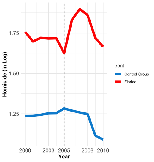
Assessing the Parallel Trends Assumption in Florida

Before the 2005 CDL expansion, Florida's log homicide rate was mostly flat, with a slight dip from 2004 to 2005. Whereas the control group remained relatively stable, with a slight uptick from 2004 to 2005. Because the slopes of Florida and the control group are not parallel before 2005, this DID research design does not satisfy the parallel trends assumption.

What’s more, following the CDL expansion in 2005, Florida showed a large increase in homicides from 2005 to 2007, peaking around 2007, and declining by 2010, but still largely above pre-treatment levels. On the other hand, the control group remained stable from 2005 to 2007 but then experienced a steep decline following the adoption of CDL.

This post-treatment gap could be explained by Florida’s rising rates of homicide, coinciding with control states experiencing a large downward shift in crime. When shown together, the plots suggest an increase in Florida’s homicide rate after the CDL expansion; yet any causal interpretation must include region-by-year FE and other controls – not present in this plot.

Homicide in Geogria

Assessing the Parallel Trends Assumption in Georgia

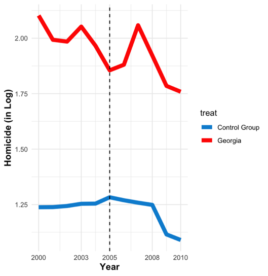
As mentioned above, the key identifying assumption in this research design is the parallel trends assumption. Due to the South historically having higher violent crime rates, Georgia has a higher average homicide rate than the control group.

On the other hand, the control group runs relatively flat, with a slight increase from 2000 to 2004, followed by another uptick from 2004 to 2005. Because the pre-trends are not parallel, it suggests Georgia was on a different trajectory before adopting the law; therefore, a simple two-group difference-in-difference would not suffice.

Furthermore, following the adoption of CDL, Georgia showed a spike in homicide rates between 2006 and 2007 before declining gradually by 2010. Whereas the rates in the control group remained flat until 2007, then declined from 2007 to 2010. The plot suggests that post-CDL, homicides increased in Georgia relative to the control group.

Altogether, this plot shows why Cheng & Hoekstra (2013) included region-by-year FE as Georgia should be compared with other southern states in the same year, rather than with a national control group.

Data Preparation for Multistate Homicide Regression

To improve the accuracy of our results, the replication exercise adds fixed effects, multiple sets of covariates and population weights to account for state-level population differences.

Why State Fixed Effects?

State fixed effects (FE) control for unobserved heterogeneity that is constant across observations belonging to a state, such as demographics (long-term racial composition, median age, urbanization levels), geography (presence of a major city, crime affected by seasonal climate), police infrastructure (officers per capita, policing style, judicial strictness, sentencing norms), baseline crime levels, cultural norms around self-defense, long-standing gun ownership rates and enduring economic differences.

These FE are baked into each state and don’t fluctuate year to year. State FE removes them as sources of bias, ensuring comparisons are within-state over time rather than across states with different baselines. In other words, state FE captures how crime changed in a state after CDL was enacted in 2005, relative to the state's crime trend prior to its passage.

Why Year Fixed Effects?

Year FE control for unobserved heterogeneity that is constant across observations that belong to all states, such as national business cycles that affect crime rates, federal sentencing revisions, and federal funding changes for law enforcement, nationwide shifts in gun culture, and nationwide declines in crime. These factors are common to all states; therefore, the replication exercise excludes them.

Basically, year FE absorbs these national shocks, so anything affecting all states each year is not mistaken for treatment effects. This is essential because crime rates oscillated in the 2000s for reasons unrelated to CDL.

Why Region-by-Year Fixed Effects?

Region-by-Year FE control for unobserved heterogeneity that is constant within each region-year, such as region-specific business cycles, regional policing cultures, regional political climates, demographic transitions, and regional crime trends. Region-by-year FE ensures that treated states are compared only to other states in the same region and year. It removes the region-specific time shocks, allowing each region to have its own baseline crime rates, distinct from those of other regions, for every year. This is critical as CDL was adopted in staggered waves across regions.

What’s more, region-by-year FE allows the Midwest, West, South, and Northeast to exhibit distinct trends each year. It also captures regional time-varying confounders (i.e. region-level variation that could dilute CDL adoption) that may mimic treatment effects, thereby undermining the credibility of the identification.

Multistate Homicide Regression

Interpreting Multistate Homicide Regression

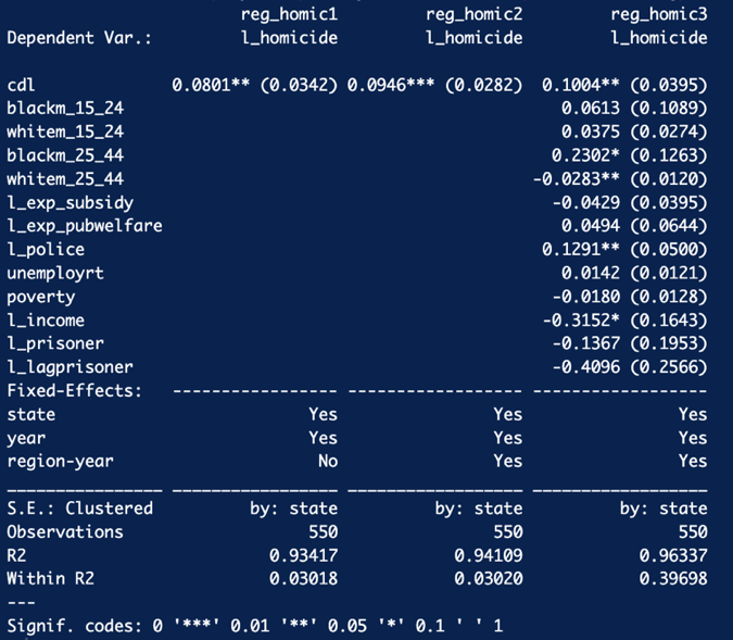
The first column considers only state and year FE, the second column adds region-by-year FE, and the third column adds time-varying covariates and state-specific trends.

After including fixed effects and population weighting, there is a statistically significant increase in homicide rates stemming from self-defense laws. This suggests that CDL increased murder by 8% when using a population-weighted regression. Sadly, this accounts for 600 additional murders per year across the 21 states where CDL was implemented. These results remain significant even as more covariates are added, but we observe a larger impact on our outcome variable, CDL, as the covariate count increases.

Alternative Model: Falsification Tests

What distinguishes an interesting paper from an exceptional one is the use of multiple sets of covariates (as shown in the multistate regression above) and alternative models (as shown below). Both ensure that estimates are robust to a wide range of econometric specifications.

For example, CDL would presumably only affect a state’s homicide rates or crimes linked to physically harming others. Crimes such as motor vehicle theft and larceny would likely remain constant during the passing and implementation of expanded laws. To test this assumption, two falsification tests were conducted.

Falsification Test: Motor Vehicle Theft

Interpreting Falsification Test: Motor Vehicle Theft

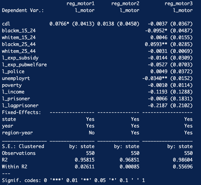
After examining the results, regardless of the covariates added, the effect of CDL on motor vehicle theft remains statistically insignificant. This provides a strong baseline for falsification tests.

Falsification Test: Larceny

Interpreting Falsification Test: Larency

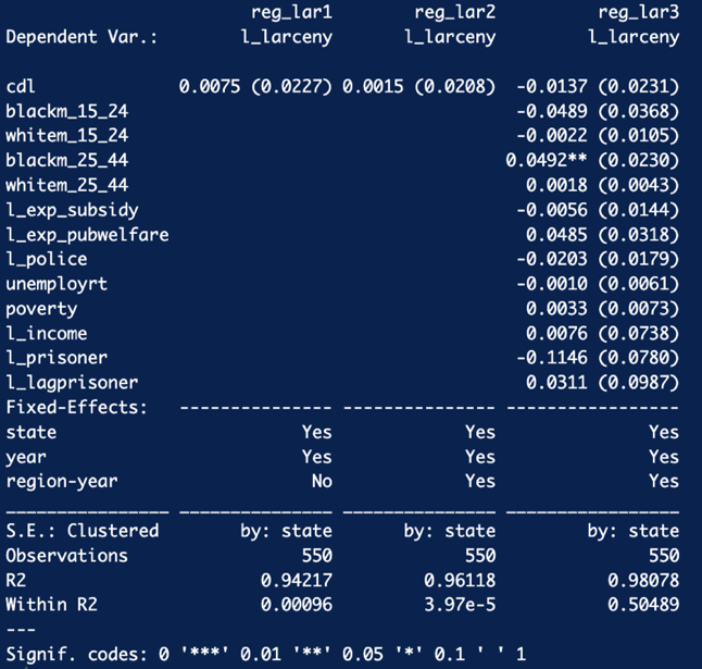
Delving into the results of this regression, once again, regardless of the covariates added, the effect of CDL on larceny (i.e. theft) remains statistically insignificant. Once more, this serves up a strong baseline for falsification tests.

Alternative Model: Deterrence Effects

Beyond testing if homicide rates change, many would like to know if CDLs have a deterrent effect. That is, if potential criminals know their victims can legally shoot them in self-defense, does that drive a drop in robbery and aggravated assault?

Deterrence Effects: Robbery

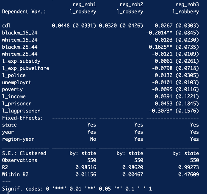
Interpreting Deterrence Effects: Robbery

According to the regression results, CDL has no effect on robbery. Because the results are statistically insignificant, they indicate that the law did not deter.

Deterrence Effects: Aggravated Assault

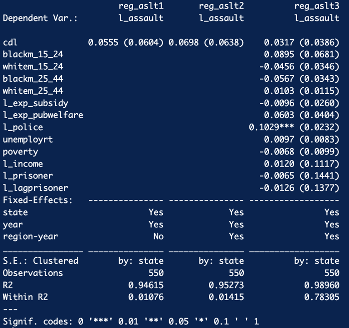
Interpreting Deterrence Effects: Aggravated Assault

The regression results show CDL has no effect on aggravated assault. Once more, the results are largely statistically insignificant and indicate the expanded law did not have a deterrent effect.

What Do Opponents of the Expanded Law Say?

While the expanded “stand-your-ground” laws do not require a person to retreat, they do not provide a blanket defense for shooting at anyone who approaches you.

Critics argue that the expanded laws make it too easy to claim self-defense when violence could have been avoided. As shown by the data replication above, there is evidence that they increase total homicide rates.

With deep gratitude and appreciation for your visit!

- Michael

Data Cleaning / Data Analysis Code